Demand and Supply

Demand: The willingness or ability of a consumer to purchase a certain good or service at any given price at any given time.

Supply: The willingness or ability of a producer to purchase a certain good or service at any given price at any given time.

Relationship between Demand and Price

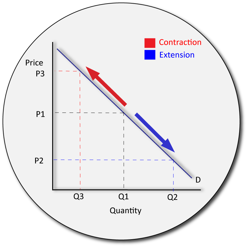
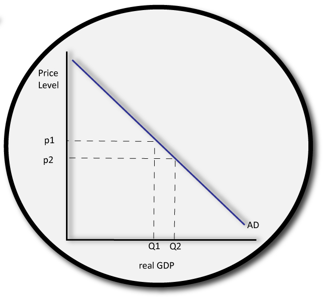
As price increases, we desire to buy less goods and services; there is an inverse relationship between the amount (quantity) demanded and the price. This is known as a contraction in demand.

As price falls, we desire to buy more goods and services; there is an inverse relationship between the amount (quantity) demanded and the price. This is known as an extension in demand.

Relationship between Supply and Price

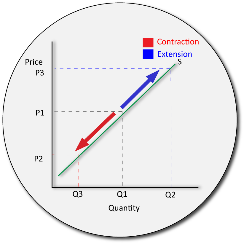
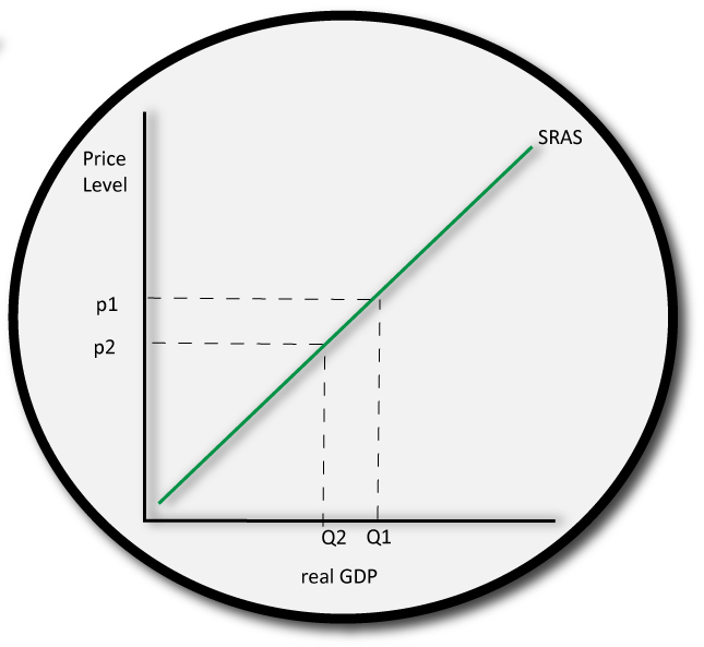
As price increases, we wish to sell more goods and services; there is a direct relationship between the amount (quantity) supplied and the price. This is known as an extension in supply.

As price falls, we wish to sell less goods and services; there is a direct relationship between the amount (quantity) supplied and the price. This is known as an extension in supply.

Shifts in Demand

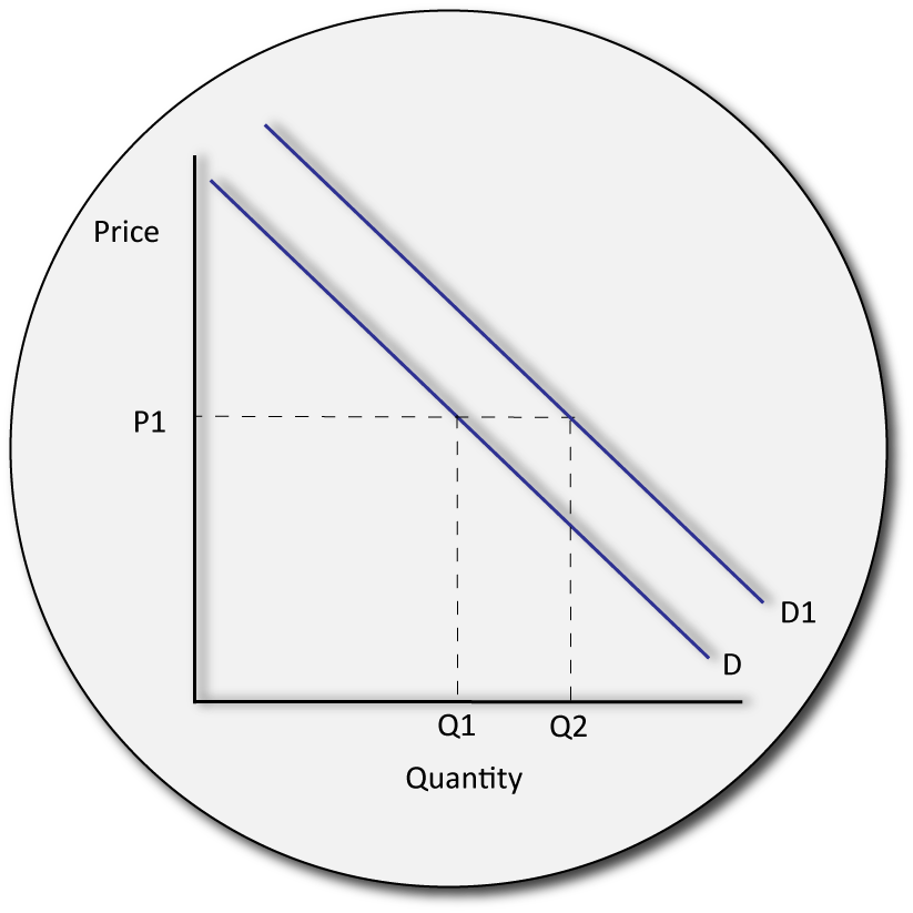
Any factor (or 'determinant') that causes us to want more or less, even though price has not changed, causes a shift in our entire demand curve. This is autonomous of price.

Determinants of demand include:

• changes in income,
• changes in direct taxation,
• changes in fashion,
• changes in population,
• future predictions,
• the price of substitute or complementary goods
• changes in perceived wealth.

When we consume more even though price has not changed this is an increase in Demand, and shown as an outward shift of the curve. (D-D1 on the diagram to the right)

When we consume more even though price has not changed this is a decrease in Demand and shown as an inward shift of the curve. (D1-D on the diagram to the right)

Shifts in Supply

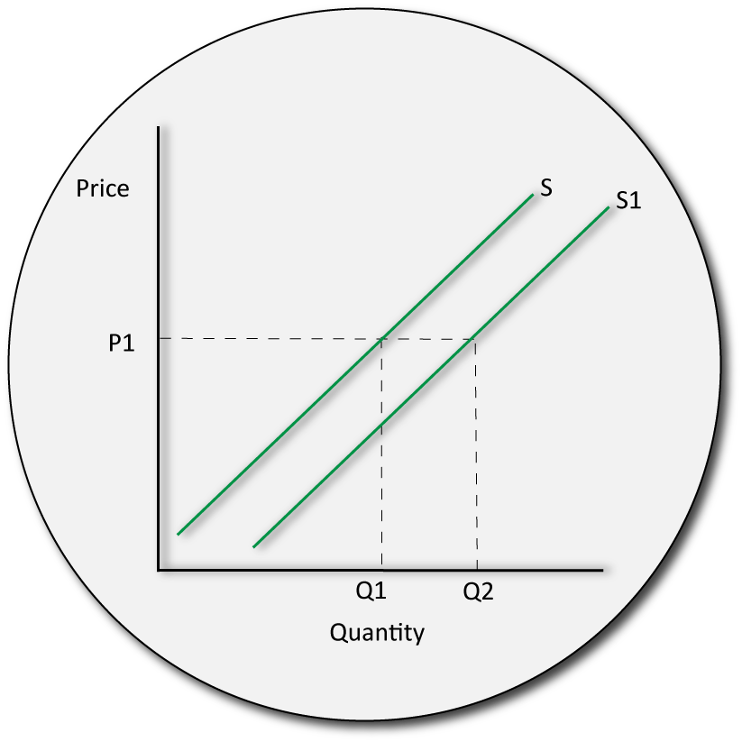
Any factor (or 'determinant') that causes producers to supply more or less, even though price has not changed, causes a shift in our entire supply curve. This is autonomous of price.

Determinants of supply include: changes in weather, changes in business taxation, changes in the costs of production and changes in red tape

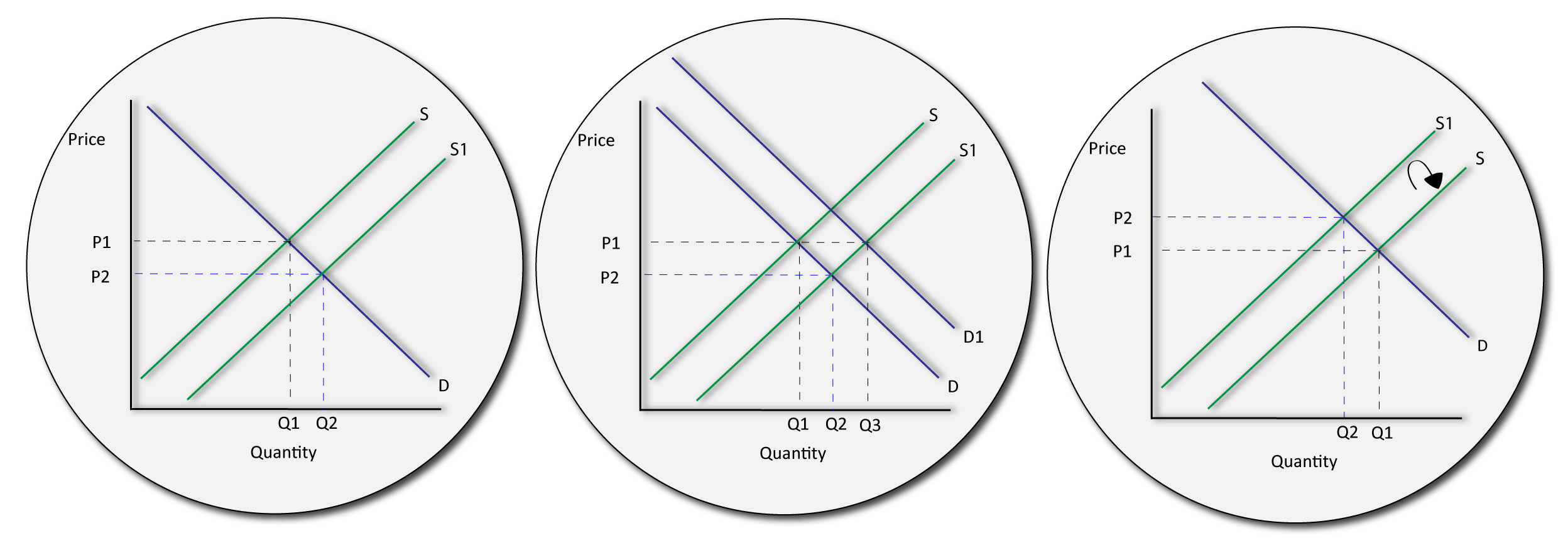
When we supply more even though price has not changed this is an increase in Supply, and shown as an outward shift of the curve. (S-S1)

When we supply more even though price has not changed this is a decrease in Supply and shown as an inward shift of the curve (S1-S)

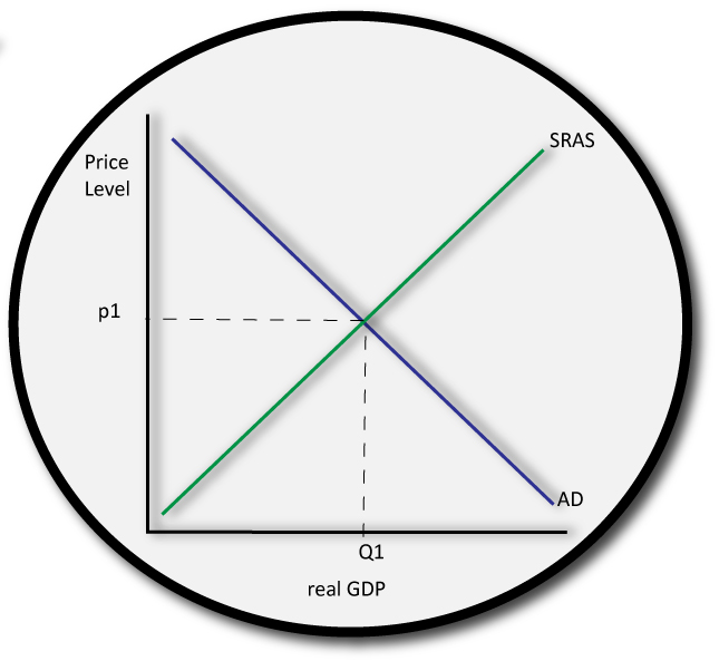
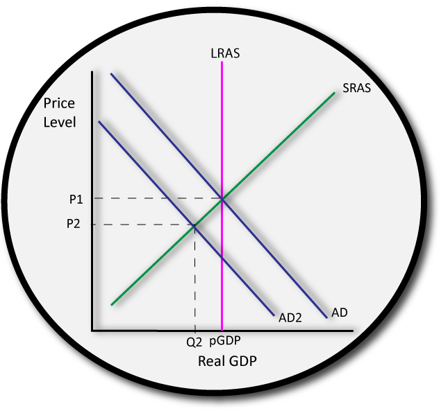
Equilibrium

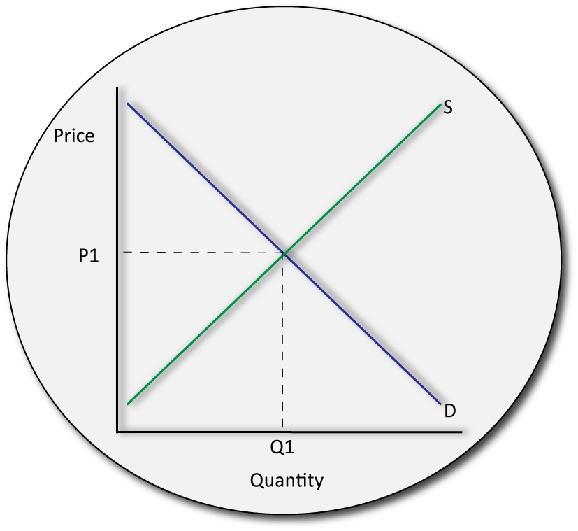
When producers agree to sell at a price that consumers are willing to buy at, this is known as equilibrium or market clearing price (P1 on the diagram to the right)

Shifts in Demand or Supply cause equilibrium price to change; this is known as the price mechanism, as explained below.

The Price Mechanism

Price acts as a signal and incentive to producers and consumers. Once equilibrium price is established both consumers and producers are content. However, a change in Demand or Supply will have knock on effects.

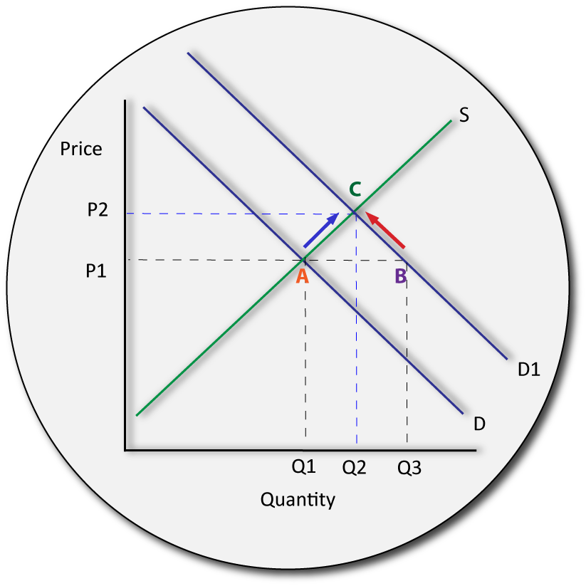
Imagine we are at Point A (Equilibrium starting price).

In this scenario lets say we are talking about the demand and supply of wheat.

If there happened to be really good weather one month, then wheat suppliers may experience an increase in the amount of wheat they can sell. Supply has shifted outwards (S-S1)

In the immediate run, if producers continue to sell at the original price, they will find that there is too much wheat on the market and that demand has already been satisfied (Point B). There is excess supply.

Instead, in order to get rid of the wheat, they must drop their prices. Wheat is now less valuable.

A change in price, however, alerts consumers. According to the Law of Demand, when price falls, consumers' demand extends.

At the same time, some producers find that it is no longer profitable to supply at this decreased price and so no longer grow wheat. Our allocation of resources has changed.

We thus end up at Point C; a new market equilibrium.

Price has acted as a signal and incentive on what to consume and produce. Price mechanisms work for any shift in demand and supply.

Excess Demand

This refers to when price remains below equilibrium, thus causing consumers to want more than is supplied. Producers will realise that they can raise the price of their product, causing a contraction in demand and a return to equilibrium

Excess Supply

This refers to when price remains above equilibrium, thus causing consumers to want less than is supplied. Producers must then drop the price of their product in order to get rid of it, causing an extension in demand and a return to equilibrium.

Applied Economics

Ever since the dawn of time, Man has always had a hankering for gold. Initially used as a form of payment, it is gold's scarcity that makes it so attractive. For example, the Spanish conquistadors were initally more interested in silver, but once they realised that by hoarding so much out of South America, they caused its value to plummet, it was gold that once again rose to prominance. The fact that it is impossible to create, and very hard to find, means that demand for gold is always high.

In fact, since 2008, gold has continued to see a resurgance in popularity - this was mainly because people began to lose faith in banks and investments, so turned instead to the shiny metal. The effect of this increase in fashion? Soaring prices of gold, of course. As of 2013, $1324/oz. Before the 1970s, all currencies were 'pegged to gold' to give them real value - for example, if you lived in the UK you could go to the bank and exchange your Pound Sterling, for a pound of gold. This will be explored later in Unit 3.

Exceptions to Demand

Several goods 'defy' the Law of Demand and have a direct relationship with price instead of an inverse one.

1) Veblen Goods -experience a direct relationship between price and quantity demanded. This is owing to 'snob-value'; a phenomenon which states that a higher price is indicative of a more expensive good, and therefore improves your social standing. Diamonds are often cited as an example; if the price of a diamond were to rise, people may want more, as they would be seen as of a higher class for buying the expensive ones.

2) Giffen Goods- although controversial amongst economists, Robert Giffen argued that certain goods in poor income families had a direct relationship between price and quantity demanded. If you take bread (or any staple) as an example: Imagine a poor family buys 3 loaves of bread and some chicken. The price of bread begins to rise. Now they can't afford the 3 loaves but must make a choice between continuing to buy the food that will sustain them (the bread) or buying less of it and continuing with the more luxurious product (the chicken). Clearly they will choose the bread and give up the chicken. With the leftover money they will continue to buy bread to make up for the chicken.

3) Goods with Expectations - as the price of some shares and stocks rise, people want more of them - as long as they believe the price will continue to rise. This is because they feel that buying more of the product at a rising price may give them better returns in the future. They expect the shares to continue rising and thus buy more of them. On the other hand, as the price of shares fall, people want less of them if they believe that its value will continue to fall. Price and Quantity Demanded are thus directly related.

Exceptions to Supply

Several goods 'defy' the Law of Supply as they have a limited relationship with price.

1) Goods/services with limited capacity - concerts can only hold a certin amount of people. It is impossible to put more than the seated capacity into the venue. Supply is thus perfectly inelastic. It is fixed and cannot be changed. Similarly, domestically, the amount of money in the economy is fixed by the government; we cannot print more even if we want to.

2) Goods that are no longer produced - you cannot reprint a famous stamp or produce more Roman coins. These goods are fixed in supply owing to the fact that it is impossible to reproduce them.

Linear Demand and Supply

Linear Demand and Supply Equations

• Linear Demand equations help us construct a demand curve using the following formula.
• Qd = a - Bp
• To work out the demand curve we do the following:

  If Qd=100 - 25p

• First we set Qd as 0, we can work out what price would be. so:
  0 =100-25p
  25p=100
  1p=4

When Qd is 0 then p is 4. 

• We then go back to the equation and now set price as 0
•  Qd = 100-0

When P is 0 then Qd is 100.  This can now be plotted

 

General Rules

When the a variable remains constant but the B variable changes, we see a change in gradient/elasticity

When the B variable remains constant but the a variable changes, we see a shift in demand

Linear Supply Equations

• Supply Linear Equations—We know that price and quantity have a positive relationship for supply We can now also see how to plot this using a linear demand formula: Qs = c+dP

  First, draw the axis for a supply diagram.

  Then, look at your equation (example: Qs= —30+20p)

  Let’s assume we want to know price (p)
  We need to rearrange the equation

  Qs= —30+20p
  Let’s assume QS=0.

  If that were true then we have the formula:  0 = —30+20p
  But this is unbalanced.  To balance it we move —30 across, our equation becomes  +30 = 20p
  To find P when QS is 0, we must therefore divide 30/20  =1.5

  Once we know price we need to go back and find out Qs

  Qs= —30+20p
  To do this, we got back to the original equation and set P at 0

  Qs=—30+0
  

  Qs= —30

  So we know that:

  When QS is 0 then P     =  1.5
  When   P  is 0 then QS =    —30
  So plot your curve!

  When the c variable remains constant but the d variable changes, we see a change in gradient/elasticity

  When the d variable remains constant but the c variable changes, we see a shift in supply

Finding Equilibrium

• To find equilibrium simply do the following: take the two equations and solve them!
• e.g: Qd =100 - 25p; Qs = —30+20p
  
  100-25p = - 30 + 20p
  130 = 45p
  p = 2.89
  
  
• We then take equilibrium price, drop it into either the Qd or the Qs equation and calculate equilibrium quantity. e.g.
  Qd = 100 - 25(2.89)
  Qd = 78
  
  
• So at equilibrium, price is 2.89 and quantity is 78

Allocative Demand and Tax Burdens

Consumer surplus can be defined as the satisfaction a consumer gains from not having to pay the price he or she was originally willing to pay. Instead, by paying the lower market (or equilibrium) price, he or she 'gains' the difference.

Producer surplus can be defined as the satisfaction a producer gains from not having to sell at the price he or she was originally willing to sell out. Instead, by receiving the higher market (or equilibrium) price, they 'gain' the difference.

Efficiency

Marginal Benefit the benefit a consumer gets from a product increases as price falls

Marginal Cost the cost to a firm of producing the next unit

Efficiency - producing using all of our resources to the maximum

Allocative Efficiency - this is where consumer and producer surplus are maximized as what is produced is reflective of society's wants. All resources are allocated according to what is demanded and can be supplied. It should also occur where p=mc (see unit 1.3 for more on this)

Productive Efficiency - where firms produce the maximum possible amount using the least amount of resources.

Economic Efficiency - where allocative and productive efficiency are met accross all markets in an economy.

Different Elasticities

Elasticity measures the responsiveness between two variables when one is changed.

The Types of Elasticity

1. 1. Price Elasticity of Demand
2. 2. Income Elasticity of Demand
3. 3. Cross Elasticity of Demand
4. 4. Price Elasticity of Supply

Each of these elasticities is useful for producers for differing reasons.

Price Elasticity of Demand

Price Elasticity of Demand—measures the responsiveness between a change in price and the effect on quantity demanded. Measured using formula below.

Price Inelastic

—tells us that a great change in price results in a small change in quantity demanded. Has a PED of <1. Usually goods with low starting price or necessities

Price Elastic

—tells us that a small change in price results in a large change in quantity demanded. Has a PED of >1. Usually luxuries or goods with many substitutes

Varying Price Elasticity of Demand—all demand curves show us varying degrees of elasticity at different price ranges. We cannot use a single demand diagram to show us elasticity in general; it must be at a specific price. Only if demand curves share a price range and intersect each other can they be compared—and even then, only at that price.

Reasons why PED is important

• Revenue Maximization—Revenue = PxQ. Producing at Unitary Price Elasticity = greatest total revenue.
• Price Discrimination— different people have different PED’s for certain products; we can maximize revenue totally by targeting different prices at different people.
• Tax maximization—To maximize taxation revenue—taxing inelastic goods producers higher government revenue
• Commodity Agreements—To ensure fair prices for commodity producers— decreasing supply = increasing TR for commodity growers—this is illogical and must be corrected

Income Elasticity of Demand

YED (Income Elasticity of Demand)

Theory: measures the relationship between a change in income and the change in demand for a product

Example: Changing incomes

Effect: The greater the positive result, the greater the shift outwards. If it is negative this indicates inward shift (and thus inferior goods)

Equation: YED = % Change of Income / % Change in Demand for Good X

Can be shown with income on Y axis, and Demand on X axis

Reasons why YED is important

• To identify sectoral change
• For investment purposes
• To show why government intervention is needed for commodity producers

Cross elasticity of Demand

XED/CED (Cross Elasticity of Demand)

Theory: measures the relationship between a change in price for one product and the change in demand for another

Example: Coke and Pepsi, Cars and Oil

Effect: The greater the positive number, the more the good is substitutional. If the number is negative, they are complements

Equation: CED = % Change of Price for Good X / % Change in Demand for Good Y

Reasons why CED is important:

• To understand internal pricing
• To understand impact on rivals
• To decide whether to merge
• To prevent from external shocks

Price Elasticity of Supply

Theory: measures the relationship between a change in price and the change in supply for a product

Example: Growing wheat.

Effect: The greater the result the more elastic supply is. If the number is <1 it is inelastic, >1 elastic.

Equation: PES = % Change in Price for Good X / % Change in Supply for Good X

Reasons why it is important:

Shows how quickly producers can react to a change in price.

Inelastic Supply

elastic Supply

Revenue and Elasticity

Revenue and Elasticity

• Between two prices every Demand curve actually has 3 sections: an elastic, inelastic and unitary elastic section.
  
  
• If producers calculated their product's elasticity they would be able to know where to set the price to maximize revenue.

• The upper section (from the middle upwards) of a Demand curve is the elastic section. Along this section, if producers attempted to increase price, they would see quantity demanded of their product fall by a greater amount. Since Revenue is Price x Quantity, if quantity falls by a greater amount than price rises, revenue will be lost.
• Along this section the producer must thus decrease prices to increase revenue (a fall in price will correspond to a greater increase in quantity demanded; thus increasing revenue)

• The lower section (from the middle downwards) of a Demand curve is the inelastic section. Along this section if producers attempted to increase price, they would see quantity demanded of their product fall by a smaller amount than the price increase. Since Revenue is Price x Quantity, if quantity falls by a smaller amount than price rises then revenue is gained.
• Along this section the producer must thus increase prices to increase revenue.

Tax and Elasticity

Price Elasticity of Demand and Tax

Knowing the Price Elasticity of Demand and Supply for our product is very useful for the government too. By working it out, they can decide on how much tax to charge. Let's look at the first diagram.

Demand here is price inelastic (<1). What happens then, when a tax - (remember, tax is a determinant of supply and thus shifts it inwards because it is more expensive to produce) - is placed on the product?

Now let's have a look at diagram 2 and at what happens if demand is price elastic (>1) and we put that tax on.

Clearly in this example we lose 30% of our product for 10% incraese in price. Q1xP1 is thus smaller than Q2xP2. Whilst the government does till get tax, this tax is lower than for an inelastic good.

Elasticity, Taxation and Consumer/Producer Burden

What about if we wanted to find out who was affected most by these taxes? We call this the tax burden - the section of society that pays for most of the tax. In an ideal world for producers, if the government put a 10% tax on a good, then they would charge 10% more for their product. They would actually then pay none of the tax, the consumer would pay it all. But to do this, their PED would have to be perfectly inelastic... unlikely.

• The way we calculate where the burden of tax falls is simple. Draw in P1 and Q1. Then draw in the effect of the tax (S-S1). Then, at the new equilibrium (marked A) draw a dotted line down to the original supply (B). The difference betwen A and B is the value of the tax.
  
  
• But B is lower than the original price. This area (green) is thus the amount of tax the producer pays. The difference between P1 (original price) and the new equilibrium price (which you can label P2) is the amount of tax WE pay.

Overall Rules

• When demand is price inelastic and a flat rate tax is imposed, the greater the consumer burden of tax- we say that the incidence of tax falls on the consumer.
  
  
• When demand is price elastic and a flat-rate tax is imposed, the greater the producer burden - we say that the incidence of tax falls on the producer.
  
  
• The more inelastic the product, the more the consumer pays the burden of tax and vice-versa.

Price Ceilings, Floors and Buffer Stock Schemes

Price Ceilings - when price is not allowed to rise above a certain limit. If set below equlibrium, this is known as a constraining price ceiling; if not, it will have no immediate effect.

Price Floors - when price is not allowed to fall below a certain limit. If set above equlibrium, this is known as a constraining price floor; if not, it will have no immediate effect.

Effects of a Price Floor

Black Markets may occur as producers seek to get rid of excess stock

Misallocation of resources - we experience excess supply

Storage problems - if done with agricultural products, we have difficulties keeping them products from going to waste

Increased income for producers, making them better off

Higher prices for consumers, causing a lack of demand

Avoidance - producers may try and avoid the price ceiling by sub-dividing products (e.g. housing if there is a price floor on rent)

 

Effects of a Price Ceiling

Long queues and lines - consumers greatly desire the product at such a low price

Lack of supply - producers gain less revenue from their product and so supply less as a result.

Black markets - consumers are so willing to buy the product they may offer a little more money in exchange for the good

Non-price allocation of resources - such as favouritism occurs, as there are few goods

Buffer Stock Schemes

Producers of commodities often face volatile (changing) prices owing to fluctuations (changes) in supply because of weather patterns. For example, rice grows very well when there are heavy rains, but suffers greatly if there is a dry season. As a result, it is very difficult for farmers to plan their incomes and lives when supply (and therefore revenue) is constantly changing.

It is obviously very bad for society if farmers start deciding to not grow crops owing to its fluctuating prices. Instead, in order to make sure enough is grown at a fair price, the government may step in and implement a buffer stock scheme. These became very popular amongst developmental economists in the 1970s, in developing countries, but have since faded in popularity.

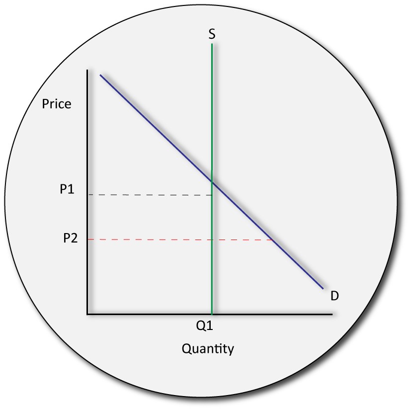
The way the schemes work depends upon many assumptions. Let us imagine that we are a rice grower and there has just been heavy, heavy rains. Supply has increased greatly and therefore, on diagram 1 below, prices fall from p1-p2 and our revenue also falls. The government though, signs an agreement with us beforehand to promise that no matter how great the increase in supply, they will guarantee us Price 1.

In order to fulfill their promise, the government then buys a lot of our rice, forcing demand back up and regulating prices. We are therefore back at p1 in our second diagram.

The next year, when a bad harvest occurs due to, say, bad rains (S-S1), prices rise. But again, the government promised us p1 and so releases all the rice it previously bought back onto the market (S1-S on diagram 3). This has the effect of lowering prices back to the agreed price and gets rid of the government's stored rice too. In this way prices have been regulated to ensure they are stable.

Problems with Buffer Stock Schemes

• Storage
• Continuous years of surplus or of bad weather
• Allocative and Productive Inefficiency
• Calculating Demand
• Agreeing an original price and time
• Government Debt and Opportunity Cost

Calculating Burdens and Subsidies

Calculating Burdens with a Tax

Indirect Tax - a tax on a good or service. Includes:

Ad Valorem Tax- a tax charged as a percentage

Flat Rate Tax - a tax charged as a specific value

• When a tax is imposed each unit of production is more expensive to produce
• This is because costs of production have now risen
• As a result, less is produced; there is a shift in supply (S-S1)
• The value of the tax per unit is the vertical difference between the two supply lines
• We calculate this by first marking on the original equilibrium price (p1)
• Then, we shift supply inwards to show a fall in production
• The vertical difference starting from the new equilibrium shows us the value of the tax

• The red area shows us the difference between the new price (p2) and the old price (p1)at the new quantity for the consumer. This is their new, reduced, consumer surplus.
• The green area shows us the difference between the new price gained (p2) and the rest of the tax (p3)
• Clearly in this case the consumer has paid some of the tax burden, whilst the producer has paid the rest.
• The amount of tax paid depends on the products' elasticity (see unit 1.2)

Understanding Market Failure

• Market failure can simply be defined as the process by which the free economic market, when left to demand and supply, fails to correct problems that the system generates.
  
  
• These 'problems' are called 'externalities' and can be defined as when a third party - someone who was not involved in the original action - is harmed or overally benefited by that action.
  
  
• There are different types of externalities. Negative externaliteis are harmful to third parties, positive externalities are unfairly beneficial.

• If the externality is caused by us - the consumers - it is a consumption externality. If it caused by a producer it is a production externality.

To understand how to draw externalities on a diagram we change our demand and supply a bit and re-interprate it.

Demand - how much we are willing to pay - becomes our Marginal Private Benefit (if we were willing to pay $10 for a t-shirt, the benefit we get from it can be shown as $10)

Supply - how much we are willing to produce - becomes Marginal Private Cost.

This is seen in the diagram.

Negative Externalities

Negative Consumption Externalities (NCE's)

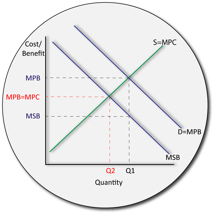
Explanation:  When consumers buy a cigarettes, the benefit to society is lower than the benefit to the individual (in this case, society is harmed by all the second-hand smoke). 

There is a separation between Private Benefit and Social Benefit.  If a good benefits the individual more than society, the individual’s satisfaction is coming at the cost to society. 

In other words, MPB is lower than MSC.  We need to encourage less people to buy these products. 

There is an over-allocation of resources so we are not being allocatively efficient.  We should be at Q2, but are at Q1.

Methods to address this: Advertising, Taxation, Legislation

Negative Production Externalities (NPE's)

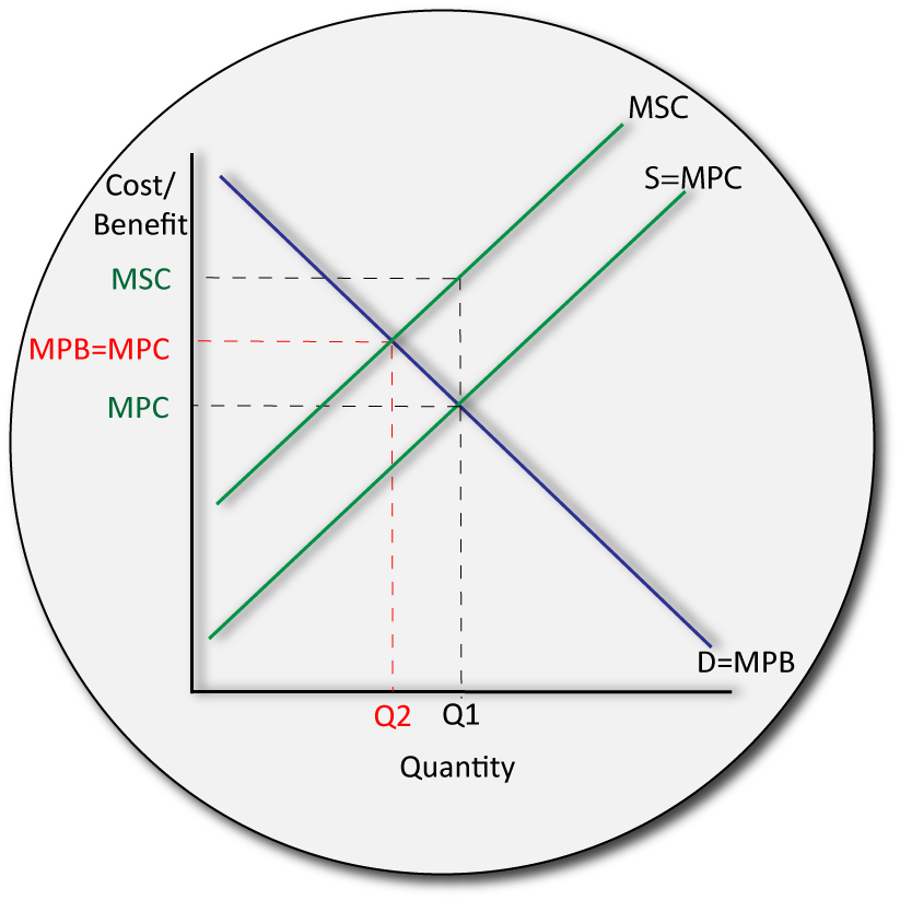
Negative Production Externalities.
Example:  Pollution.

Explanation:  When a firm pollutes, the cost to society (in the form of all the healthcare costs) is greater than the private cost to the firm.  The firm does not care about the pollution, but everyone else suffers.  Society wants us to produce much less (Q2) but we are over-producing this good (Q1).  There is a separation between MPC and MSC.  We need to find a way to correct this.

Methods to address this: Pigovian Taxes, Trading Permits, Laws, Property Rights

Positive Externalities

Positive Consumption Externalities (PCE's)

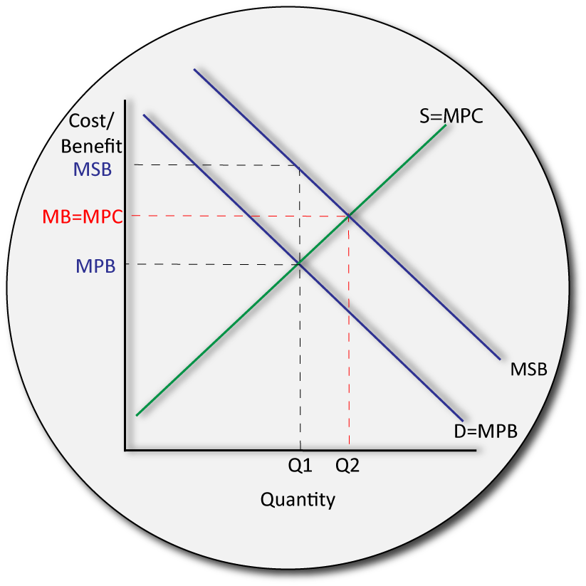
Positive Consumption Externalities.
Example:  Buying a hydro-electric car

Explanation:  When consumers buy a hydro electric car, the benefit to society is greater than the benefit to the individual (in this case, society benefits from all the clean air).  There is a separation between Private Benefit and Social Benefit.  If a good benefits society more than the individual, the individual will not be inclined to buy as much of it as society likes, as his personal satisfaction is not great enough.  In other words, MPB is lower than MSC.  We need to encourage more people to buy these products.  There is an under-allocation of resources so we are not being allocatively efficient.  We should be at Q2, but are at Q1.

Methods to address this: Advertising, subsidies, legislation

Positive Production Externalities (PPE's)

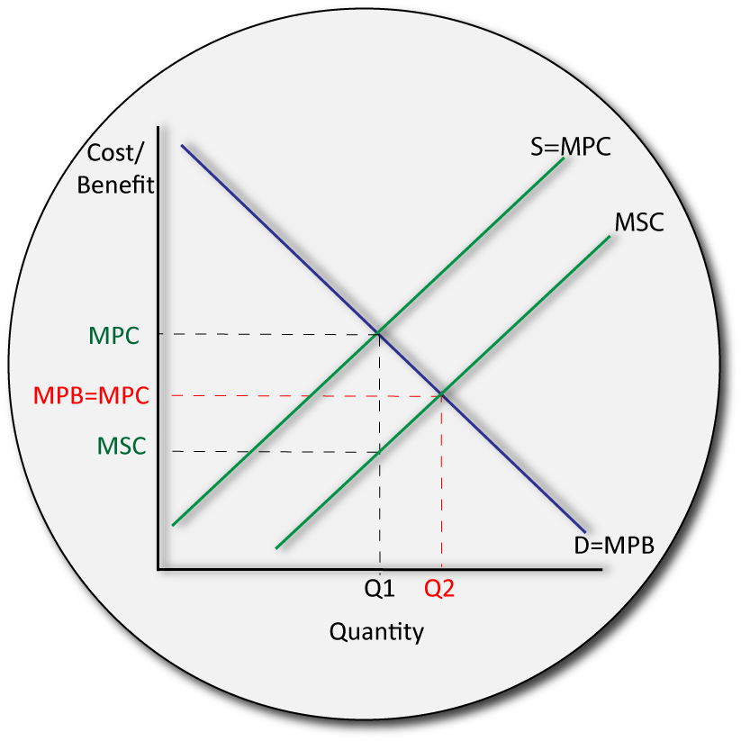
Positive Production Externalities.
Example:  Research and development of drugs.

Explanation:  When producers pay millions of dollars to discover a new way of doing something, then all of society benefits greatly.  However, the firm itself paid a high cost (millions of dollars) for the research.  If everyone gets more benefit from the research than the firm itself, it is unlikely to continue doing such research.  There is a sepeartion between the cost to the individual firm, and the cost to society.  We need to somehow encourage the firm to continue producing their goods as society wants Q2 but we are only at Q1.  There is an under-allocation of resources so we are not allocatively efficient.

Methods to address this: Subsidies (increases S=MPC so that S=MPC=MSC)

The Trade Cycle

• This attempts to explain the general ebb and flow of macroeconomics.
  
  
• To put it simply, economies experience good times, followed by bad times, followed by good etc.
  
  
• Where we are in that cycle depends on our real GDP growth. World history has shown us that the general trend for all countries is for there to be a general increase over time, punctuated with highs and lows.
  
  

• We must also understand the concept of the 'natural rate of unemployment'. If we look at the Trade Cycle, we can see that we are able to produce above our potential real GDP. This, surely, makes no sense: how can you produce more than you are able to produce??
  
  
• The answer lies with the natural rate of unemployment. This states that in every economy we want to have around 3% of unused factors of production. This is because it helps the economy remain fluid (workers can replace other workers, land has time to recover etc).
  
  
• If we use these resources, we therefore have a lower rate of unemployment than we should do - an inflationary gap.
  
  
• If we use less than 3% we have more unemployment than the natural rate - a recessionary gap.

Measuring Economic Activity

When starting our Macroeconomics Unit, we need to first familiarize ourselves with the terminology of what we are actually studying. What Macroeconomics is all about is the whole economy - all of it - and how well or poorly it is doing.

That's quite a lot to look at.

• As economists, we narrow down the basic health of an economy (or 'economic growth') to being how much GDP has grown.
  
  
• In order to help us understand what GDP is, we generate what is known as the 'Circular Flow of Income Model'. Have a look at it below.
  
  
• What the diagram shows us is simple. We - as people - trade our factors of production (in this case labour) for money, in the resource market. We go to work and receive income.
  
  

• We then spend that same income and receive goods and services (in this example a car) in return.
  
  
• What does this show us? Well, in a perfect economy, the amount we receive in wage is equal to the amount we spend on goods and services, which is equal to the value of the good/service.
  
  
• Think of it this way: if a producer knew he gave you $100, he would set the value of his car at $100 and then you would have to spend $100.
  
  
• As a result:

National Income = National Expenditure = National Value of Goods and Services.

• When we talk of measuring economic growth, we can therefore calculate any of the above and reach the same conclusion - theoretically.
  
  
• As economists, it's easiest to calculate National Expenditure. We do this by adding together what everyone in the economy has spent - or bought. We first divide the economy into four purchasing groups:
  
  
  • Consumers - buy goods and services
  • Investors - are businesses who usually buy capital
  • Governments - who pay for merit goods and public projects
  • Exporters and Importers - we calculate how much we gain from selling abroad, and how much we spend abroad.
  
  
• This can be written as:
  C+I+G+(X-M) Consumption + Investment + Government Spending + (Exports - Imports)
  
  
• The total value of goods and services in a country in a certain time frame can thus be generated using the above knowledge. Quite simply C+I+G+(X-M) is just the easiest way to calculate Gross Domestic Product (the value of final goods and serives in a country in a certain time frame). It's the same thing.
  
  
• GDP is thus our yardstick for measuring economic growth. But the problem is there are many types of GDP:
  • GDP—(Gross Domestic Product): the value of all goods and services produced within a country in a given time frame
  • GNP (Gross National Product) —the value of all goods and services produced by a country’s citizens in a given time frame
  • GDP per capita—the value of all goods and services produced within a country in a given time frame divided by the population
  • NDP—Net Domestic Product—the value of all goods and services produced within a country in a given time frame, minus depreciation (money spent on replacing capital)
  • Purchasing Power Parity GDP

• We must also be careful to stress the FINAL aspect in GDP.
  
  
• Final goods and services, means that we calculate their value when they are sold at their last use.
  
  
• We do not add up all the values before this, as these values are already hidden in the final value as costs. Look at the
  Life and Times of Tim the Chicken for more clarity.

• The main economic growth indicator we use is Real GDP per capita. We take it as a %.
  
  
• In order to make it a %, we need two different time frames to compare it to. You can't say real GDP per capita in 1999 was 2.2%... what does that mean?? But you can say real GDP per capita increased by 2.8% in 1999 from 1998.
  
  
• We therefore use the following formula:
  Economic Growth = GDP Indicator Final Time Frame - GDP Indicator Orginal Time Frame /divided by GDP Indicator Original time frame
  
  
• We call it 'Measuring National Income'. Really, we could call it 'Measuring National Expenditure' or 'Measuring National Value of Goods and Services' - it doesn't matter, they should (barring statistical differences) give us the same answer. GDP is just the easiest way to measure national income, and thus economic growth.

Problems with Measuring Economic Growth

through National Income Statistics

• Statistical discrepencies
• Difficult to compare over time (as incomes generally rise)
• Difficult to compare accross coountries
• Difficult to assess living conditions
• Cannot discern Purchasing Power

Welfare and GDP

welfare

• Welfare can be defined as the general living standards in a country. It takes into account the comfort, or happiness of the population, as well as its economic activity.
  
  
• It cannot be measured using GDP, but is instead a subjective view

How GDP under-emphasises welfare

• Does not take black market into consideration - Greece in 2012 is often cited as having very low levels of GDP, but this is not entirely true. Economists estimate that around 25% of economic activity occurs on the black (or shadow) market. This is not accounted for in government statistics, and means that the level of economic activity is higher in Greece than GDP states.


• GDP does not reflect quality - China's GDP figures have been soaring in the past few decades. Few economists doubt the level of economic growth. Germany's GDP has remained fairly constant, in comparison. Nonetheless, there is no way of differentiating the goods being recoreded in terms of quality; China's product quality has been notoriously poor, but GDP does not reflect this.
  
  
• GDP is drained by pensioners - but this is a good thing. A country with excellent health facilities will have a greater ageing population. However, pensioners often have state pensions and do not contribute to GDP as they don't work. GDP therefore seems low, even though living standards are high.
  
  
• Leisure vs GDP - Chinese workers have very long hours. Their GDP thus increases along with their productivity. Very developed countries place more emphasis on holidays and leisure time which actually reduces GDP as they are no longer in work. Still, living standards rise.
  
  
• DIY - many countries do work on their houses or cars themselves. They don't pay themselves to do this, nor are the goods they produce recorded as part of GDP.

How GDP over-emphasises welfare

GDP may be high but welfare may actually be lower for the following reasons:

• Negative Externalities - if a country produces a lot of goods and services but takes no account of externalities such as pollution, then the welfare of the country will be a lot worse than GDP suggests. As a result, Green GDP is a better measurement of welfare.
  
  
• Opportunity Cost - or cost taken into account in order to have rapid GDP is often forgotten. China may have high levels of GDP but this came at a cost of losing natural resources and habitats.
  
  

Why GDP is misguided

• Who earns the GDP?

A country may look like it is growing considerably, but this may not be true if all the GDP is earned by a single person (such as an oligarch).

• What is the GDP made up of?

  North Korea may seem to have a high level of GDP but this would be misguided: Most of the money is spent on arms and weapons related industries, which does not really reflect a growing economy - GDP does not indicate this difference.

  
  
• Lacks social indicators- increasing the value of goods and services doesn't actually mean people are better off; we know little to nothing about important welfare measurements such as life expectancy and birth rate.
  
  
• PPP is not accounted for

  countries may have a high value of goods and services, but if Purchasing Power Parities are not accounted for then it is hard to compare their GDP with other countries. PPP simply use economic formulas to see how far a person's income would go in the US. A country could thus have a real GDP per capita of $50 000 but a PPP real GDP per capita of $100 000; this shows us that their money can go twice as far as in the USA.

Other Measurements of Welfare

1. Human Development Index.

This is a composite indicator that includes three aspects of living standards to create a score between 0 and 1. The closer the overall score to 1, the higher the living standards. The current three indicators are:

• Life Expectancy (this is the health element)
• Education (this is the living standards element)
• National Income Levels (this is the GDP element)

Aggregate Demand and Supply

Aggregate Demand Explained

Aggregate Demand is different to demand for just one good or service. Aggregate literally means 'overall' or 'composite'. When we talk of aggregate demand, we are looking at the whole economy, not just one good or service. We are looking at what demand is like for ALL goods and services over a given time period.

Because we are looking at aggregate demand, the axis for our demand diagram changes. We are not looking at price for one good or service, but prices for ALL goods and services. We call this the 'price level' in our economy.

Also, we change quantity into real GDP. This is because the value of all things produced in an economy over a given time period is not just quantity - it is GDP (as seen through the expenditure method).

Just as with normal demand, people in our economy will buy more goods and services when the price level is lower. AD thus has an inverse relationship with price levels.

Determinants of Aggregate Demand

Determinants of Aggregate Demand are simply factors that cause an entire economy to want to buy more goods and services. AD is split into four components, each of which has its own determinants

• Consumption (C)- if people wish to buy more/less goods and services, our overall demand (AD) is affected. This could be because of
  • Changes in Incomes
  • Changes income tax
  • Changes in interest rates
  • Changes in debt levels
  • Changes in consumer confidence
• Government Spending (G)- if the government acts as a consumer and buys more/less goods and services (such as by building schools or roads or hiring more public workers) then it influences the overall demand (AD) in our economy.
  • Changes in political priorities
  • Provision of merit and public goods
• Investment (I)- producers also manipulate our economy's overall demand by investing in capital for their firms. They thus act as consumers.
  • Changes in business Tax
  • Changes in business confidence
  • Changes in interest rates
  • Changes in technology
• Exports - Imports (X-M)- if we export more than we import then more money is entering the circular flow, and thus people have larger incomes and spend more, causing AD to rise. If we import more than we export, money is leaving our circular flow, and thus AD will decrease as incomes fall. Changes in exports and imports can be caused by
  • Changes in protectionism
  • Changes in exchange rates
  • Changes in demand for imports/exports
  These will be explored in Unit 3.

Aggregate Demand is thus calculated using the equation C+G+I+(X-M). If the components yield a positive number, Aggregate Demand shifts outwards. If they yield a negative number it shift inwards.

Aggregate Supply Explained

Aggregate Supply is different to normal supply in that we are now looking at the total amount of goods and services willing and able to be produced in an economy by all firms.

Aggregate supply can be drawn as a straight line that has a direct relationship with price level (as prices for goods and services are higher, firms produce more) but can also be seen as a sloping upward curve because - at some point - resources run out so no more can be produced.

The nature of the Aggregate supply curve is controversial - different economists have different opinions on what it looks like and whether it can be split into two separate curves itself. This is explained in units below (Neoclassical vs Keynesian).

Determinants of Aggregate Supply

Factors that shift the supply-curve in the short-run occur when the price of factors of production change - if factors of production become cheap, firms can supply more at the same price (an outward shift). If they become more expensive, firms supply less at the same price (an inward shift). These changes may occur due to:

• Changes in business taxation
• Changes in the availability of resources (i.e. if oil began to run out it would become more expensive)
• Changes in wage levels
• Supply-side shocks (war, natural disasters, famine)
• Changes in the price level of crucial imported factors of production (e.g. oil)

These changes in supply are generally true for the short-run. If we wish to permanantly increase supply we must achieve the following criteria:

• Increase our factors of production
  • e.g. find new oil reserves, have a larger population that can work
• Increase the quality of our factors of production
  • e.g. education, training, efficiency
• Increase technology
  • e.g. new harvesting machinary

You will notice these are the same criteria for increasing our PPC - essentially the idea of long-run supply and PPC are the same; they show us what we are able to produce.

AD and AS in Equilibrium

Short-run macroeconomic equilibrium occurs when the forces of aggregate demand are equal to those of aggregate supply. We are producing at a price society is willing to pay, and producers are willing to sell at.

This does not neccessarily mean we are using all of our available resources in the economy - that would be long-run macroeconomic equilibrium. This is explored more in the sub-headings below.

New Classical Economics

Applied Economics - The New Classicalists

Freidrich Hayek is perhaps the most well-known of the neoclassical economists but his work built on the works of other notable names such as Alfred Marshall and Thorstein Veblan. Three assumptions (people act rationally, firms are profit maximizers and perfect information is obtainable) form the backbone of new classical thinking.

Born in Austria-Hungary, Hayek became a prominant economist in the twentieth century and based his ideas on the fact that price acted as a direct signal to firms to change wages. In the 1980s, after stagflation had left Keynesian economists bewildered (see Keyens in drop-down box below), both the USA and the UK (major world powers) adopted Hayek's free-market thinking.

The main ideas Hayek advocated was that governments needed to do less, not more, to help economies grow. The less involvement a government had, the more prices would be able to send signals to firms, which would lead to wage changes so that long run equilibrium could be maintained (see below). Margerat Thatcher certainly followed this advice by closing down the UK's mines and by deregulating many industries, famously saying "competition works".

Hayek and Keynes (discussed below) clashed many times but always held a healthy respect for one another. Hayek's ideas have formed the major thinking of post-1980s Western economics, though the banking crisis and major recessions of recent decades have led to the beginnings of a distancing from his theories.

Neoclassical economists build upon the work of the 'Father of Economics' - Adam Smith. They claim that, if left alone, the economy will always swing back into producing at potential GDP.

To understand this we must understand the following steps:

1) Aggregate Demand is more likely to fluctuate than Aggregate Supply in an economy
2) When it does move, AD changes prices
3) Prices are linked to wages
4) Wages are a cost of production
5) Wages thus influence the Short-Run Aggregate Supply curve
6) Aggregate Demand thus is intrinsictly linked to Short-Run Aggregate Supply

This relationship can be expressed below:

Short & Long Run AS

What is all this 'Short-Run' about? Well, according to their theories, there is a great difference between Short Run AS and Long Run AS. The difference is the time it takes for wages to adjust to price changes. This only happens in the Long Run, according to Neoclassical Economists. The Long Run Aggregate Supply is therefore the amount we produce when wages have been taken into account. According to Neoclassical economists, if we start at equilibrium, we will always end up there as inflationary and recessionary gaps will be taken into account naturally. Lets consider this below.

In the diagram above. We were at equilibrium (where AD met SRAS). Then, Aggregate Demand rose (for whatever reason). Prices therefore rose to P2. If Q1 was our Potential GDP, we now enter an inflationary gap. Workers therefore began to feel that life was a bit too expensive, and asked for a wage increase. If prices rose by - say - 10%, they asked for a 10% wage increase. This made it more expensive for producers to produce, so SRAS fell. We end up at P3 and Q3. Notice that Q3 is the same as Q1!

Because Q1 and Q3 are the same, neoclassicalists say that that quantity represents potential GDP, or the amount we always end up producing in the long run, no matter what happens in the economy. Or... our Long Run Aggregate Supply (LRAS).

This takes us to Diagram 2 where we reinterpret the first Diagram. LRAS is our potential GDP. Even if AD increases, we end up at our potential GDP in the long run because wages change too.

AD does not influence our long run production even if it falls, as seen below.

We see that when AD falls, prices fall in the economy (as producers have to lower them in order to get rid of the goods as less people want them). As a result, firms get less revenue. Because of this, producers tell their workers they must take a wage cut. Having taken a wage cut, supply can then increase as it is cheaper to produce. SRAS shifts outwards (to SRAS1), causing us to produce the same amount as when we started the cycle. Recessionary gaps are thus just temporary.

Keynesian Economics

Applied Economics - John Maynard Keynes

After the horrors of the First World War, Keynes saw for himself the destruction Man coul cause. The sweeping poverty, rationing, disease and disjointed economies of Europe moulded his economic thinking. Born in Cambridge, Keynes went to the prestigious Eton College before returning to Cambridge to study at its university. There, he formed a close circle of liberal-thinking friends in what became known as the Cambridge Apostles. After leaving university, Keynes became a respected economist, though his views were ignored at the Treaty of Versailles - the peace treaty after WW1. He would continue to insist that Germany needed not punishment but subsidizing if another war was to be avoided. After it, he claaimed "vengeance, I dare predict, will not limp." He was right.

The subsequent Great Depression that followed the First World War really crystalized Keynes' developing views on how economies work and neccessary solutions to combat the ills he saw. With unemployment soaring, economic growth collapsing and investment almost non-existant, Keynes believed the solution was to abandon the New Classical way of thinking - instead, an almost total reversal of policy was in need. Instead of less government spending, more. Instead of laissez-fair, interventionism. It was a government's moral and economic duty to revive countries that had fallen into deep recessions - so deep that they would not be naturally righted.

In 1936 he published his groundbreaking work entitled A General Theory of Employment, Interest and Money in which he exorted governments "Let us be up and doing"! The Second World War would interupt the progress of his policies, but after it had ended Keynesian ideas were not abandoned; instead, the USA and the UK both undertook them - Atlee in the UK created the National Health Service (NHS) whilst the Hoover Dam in the USA (completed in 1935) showed the US' commitment to Keynesian ideas.

Keynes' ideas formed the backbone of economic policies around the world from the 30's to the 70's and revolutionized the hands-off approach to New Classicalism. It would not be until the arrival of Friedman that this would all change...

Based on the works of John Meynard Keynes in the inter-war years, economists who follow this understanding of the economy have a very different view.

Their disagreement with the New Classical economists starts with recessionary gaps. Supposedly, when AD falls, prices fall and so - therefore - do wages. "Rubbish!," say the Keynesians. Wages rarely really fall in the economy - trade unions, laws and just general common sense prevent them from doing so. No, the Keynesians prefer to break the economy up into 'stages' instead of having a SRAS and a LRAS.

Below we can see the Keynesian view of the economy

What's going on here? Don't panic. The diagram above helps explain this. In the blue section on the diagram, we can see that the supply curve is horizontal. If we imagine AD was on this flat segment, and we increased AD (by shifting it to the right) there would be no change in prices. This is the opposite to what neoclassical economists say! Why is this?

Keynesians claim that in the flat section, resources are abundant, and not being used. There is plenty of land, labour, capital and enterprise lying around unused. In fact, so much is not being used that even when we demand more, the price remains low (as its abundance makes it have less value).

Only when we approach the pink section can we see prices begin to rise. Along this section, resources begin to run out (called 'bottlenecks'). As AD increases on this section, we use up our factors of production - if you want more stuff, you start to have to pay more for it, as its no longer abundant. Somewhere on this section we have our potential GDP (which includes natural unemployment).

Finally, when approaching the yellow section, we are using ALL of our resources. We cannot increase production at this point. If AD keeps increasing then we will produce beyond our potential GDP and thus enter an inflationary gap. On this section, Keynesians agree that increasing AD will only lead to increasing prices.

So, what the Keynesians believe, overall that if we are in a recessionary gap (producing below p.GDP) then we can get stuck there if the government doesn't intervene to boost aggregate demand. This is shown in diagram below.

Whilst if AD is above p.GDP then we are in an inflationary gap and AD needs to be reduced, as seen in the diagram below.

The Multiplier Effect

This attempts to explain the relationship between expansionary fiscal policy and the knock-on effects in the economy.

If the government decides to spend in the economy, their initial expenditure is known as autonomous spending. For example, if the government decided to build a road, the autonomous spending would be the amount (say, $10m) spent on that round. This would increase AD by the orange segment on the diagram to the right.

Induced spending, however, is the amount of money spent in the economy after the inital autonomous spending. In this example, after the government had spent the $10m, the road workers would take home their wages and spend it on food or clothes, or anything else. The amount they collectively spend is thus known as induced spending. This would further increase AD by the pink segment on the diagram.

It is clear then, that adding a little money into the economy causes a greater increase in economic growth. In our example above, the government may have only put $10m in, but this $10m could have been spent through the economy four more times, creating total economic growth of $10+$40m = $50m

How much induced spending is created, depends though on our Marginal Propensity to Consume. This is simply how much of the next unit of income we earn, we spend. If our MPC was 1, that would mean that we would spend all of the money given to us.

When we know our MPC, we can use the Keynesian Multiplier Equation to work out how great an increase in GDP will be caused when a government injects money into the economy. The formula is: 1/1-MPC

Once we know the Multiplier, we can then multiply it by our autonomous spending to find out how much economic growth is created overall.

Keynesians see this as useful compared to Neoclassical economists because they beleive AD can create economic growth, not just inflation.

Unemployment

Definitions

Unemployment can be defined as the amount of people actively seeking a job but who are without one.

The unemployment rate is the percentage of the labour force (those that are willing and able to work) that are without a job. It is calculated by dividing the unemployed by the labour force x100.

Difficulties in Measuring

• Underemployment
• Statistical discrepencies
• Hidden unemployment / Informal Economy
• Does not account for geographical differences
• Is all-inclusive (does not divide age, gender, ethnicity)

Types of Unemployment

1. Structural - when the skills of the workforce do not match the jobs available in the economy
2. Frictional - the type of unemployment caused as workers move between jobs
3. Seasonal- when workers have a job reliant on the weather and are unemployed in the off-season
4. Cyclical / Demand-deficient - when Aggregate Demand falls due to any reason (e.g. higher taxes) and so less workers are needed
5. Real-wage - when wages are set too high and so firms demand less of them then they would do otherwise

Causes of Unemployment

1. Structural
• Technological changes - when new technology is introduced that can do the work previously done by workers (or when human capital becomes outdated) then workers have skills that are no longer needed in society.
• Sunset industries - industries that previously were very large (such as the mining industry in the UK or the car industry in the USA) provided many jobs. However, foreign competition or a lack of demand for the goods provided by these industries forces them to close, causing wokers to have skills that are not needed.
• Geographical changes - if a firm decides to move from one part of the country to another, few workers will follow. This will leave many workers stranded with uneccessary skills.
• Changes in demand - if a country moves out of one sector of society and into another (ie from the primary to secondary sector) then the primary industry skills will no longer be needed.
2. Frictional -
• Lack of information - if workers are unaware of available jobs they will be unable to move between them quickly or easily. Countries with low internet access or poor job centre provision often suffer from this.
• Lack of infrastructure - if workers are unable to move between jobs due to poor roads or poor communication there will be higher rates of frictional unemployment
3. Seasonal -
   • Lack of information
   • Lack of infrastructure

In any economy these 3 types of unemployment are common and - to some extent - unavoidable. They will always exist to some degree, even when we are producing at long-run unemployment (as this includes the natural rate of unemployment too). As a result we call them 'natural unemployment' or 'equilibrium unemployment'.

4. Cyclical / Demand-deficient -
• Fall in AD due to government policies (deflationary fiscal/monetary policy)
• Fall in AD due to fall in determinants of C, I, G, X-M
5. Real-wage -
   • Minimum wage set above equilibrium - when the government sets minimum wage above equilibrium then there is an excess of supply of labour in the labour market. Firms hire less workers as they are more expensive, and so produce less. SRAS shifts inwards.
   • Trade union power - has the same effect as above
   • Legislation - if it is difficult to hire labour the effects will be the same as above.

These two types of unemployment are not natural in an economy and are avoidable through government policy. They occur when we are not producing at long-run equilibrium and are thus known as 'disequilibrium unemployment'.

Cyclical is shown on the first diagram below, whilst real wage is shown in the last two diagrams.

Consequences of Unemployment

• Social problems - crime, stress, depression
• Loss of GDP
• Deflation (if cyclical)
• Loss of tax revenue
• Budget deficit (loss of tax revenue AND increase in benefit spending)
• Increased debt
• Worsening income distribution

Solutions to Unemployment

Solutions to unemployment depend on the type of unemployment it is. To identify solutions we must first identify the cause. This is the reason why knowing the type of unemployment is so important.

Applied Economics: Spanish Unemployment

Since 2008, the Spanish fiscal crisis has gown exponentially. The reasons for this lie in the fact that despite enjoying a balanced budget before 2008, banks invested far too much money into 'toxic assets' such as housing. As European banks happily provided the money, Spainish banks happily spent it. When the rosy-looking house market turned rotten, the government was then forced to intervene and prop up the banks to avoid a bank-run and widescale economic turmoil. This instantly put them into debt.

Meanwhile, regional governments acted irresponsibly with the wealth they had created before 2009 - large-scale projects were built - including a new airport in Valencia, and a new arts museum in Barcelona. This would have been fine except for one thing: the projects were not sustainable. Valencia's airport cost a whopping 150 million euros but has yet to take off. Literally. No flights have gone too or from the airport, as it was both unneccessary and too expensive for airliners.

The cost of all this mis-management, which started with financial sector irresponsibility (how, as a government, do you deal with organisations that get paid to fail?!) is enormous unemployment. With austerity measures in place to pay back large debts, jobs have been sacrificed. The banks are also no longer splashing the cash, meaning nothing is trickling through to small and medium size enterprises. The housing market - and all the industry (glass makers, cement mixers, builders, real-estate agents, insurors) that comes with it - now lies dormant. Unemployment in Spain has rocketed from 7% in 2007 to 21% in 2013.

As nothing is being created, it is the young that are feeling the hit the most. Spanish youth unemployment stands at 46%. This translates into a huge cost for the government who, after spending years (at a considerable cost) educating and training their young, are simply leaving them high and dry once their education is complete. The opportunity cost is immense. And yet, the government - torn between being able to pay back its debt in order not to fall into economic ruin and being able to provide jobs through fiscal policy - are left in a sticky situation. The end result? A whole of angry, disatisfied youths (crime is on the rise) and a whole lot emigration. Germany is seen as the number one destination for the unemployed Spanish youth - followed by the UK.

Inflation

Definitions

Inflation is a sustained increase in the prices of goods and services in an economy over a given time frame.

Inflation rate is the percentage rise in the prices of goods and services in an economy over a given time frame. Even if it falls, this still shows us prices are rising, but at a slower pace.

Disinflation is a slowdown in the rate of inflation (prices of goods and services are still rising but at a slower rate or perecentage) per time frame.

Deflation is a sustained decrease in the prices of goods and services in an ecnomy over a given time frame.

The inflation or deflation rate (from which disinflation may also be calculated) is a percentage increase or decrease in the prices of goods and services in an economy over a given time frame.

Measuring Inflation

CPI (Consumer Price Index)- This is the main way inflation is calculated. To do this, the government collects around 500 essential goods and services and puts them into a hyperthetical 'basket'. The year in which it assembles the basket is known as the base year. This is usually a normal year where prices have not been fluctuating greatly

Once this is done, the prices of all these goods and services are added up but a price index is set for 100 at the base year. All this does is make it easier to compare how prices have changed over time. The following year, the prices are added up again and divided by the original price value for the base year, to work out the percentage change. If this came to - say - 10% change, the new price index for year 2 would be 110 (the orignal price index of 100 plus the new 10 percent increase). This allows us to see inflation over time easily.

There are other issues that are taken into account. Obviously, some goods and services are more important than others and affect us to a greater extent. As a result, there are different weightings given to different goods. For example, petrol/gas is given a greater weight than i-pad apps. The way weightings are worked out are simply by finding out how much of each good/service is consumed as a proportion of their income (this involves complicated economic forumlaes).

For example, if the average household buys 3 i-pad apps at an average price of $2, then the final value that goes into the basket for i-pad apps would be 3 x $2 = $6.

Similarly, if the average household buys 30 units of petrol at an avarege price of $50, the final value that enters the basket would be 30 x $50 = $1500.

Consequently, any change in petrol will affect the basket to a greater degree than any change in i-pad apps. It is only once this is done, that the final price indices can be calculated.

Be careful: economists measure inflation relative to the base year. It is possible to measure it relative to the previous year. To do this, we would simply take the price index for Year 2, divide it by the price index for the previous year and multiply this by 100.

Producer Price Index

Producer Price Indices measure changes in the price of factors of production. They work in an identical manner to the CPI, but instead of having a basket of goods and services that are regularly consumed by the average household, they have a basket of factors of production that are neccessarily used by the average business. This can be useful for predicting future inflation but its importance to developed countries is declining due to the decline of many manufacturing industries therein.

Problems with Measuring Inflation

• Does not show quality
• Is an average - does not reflect impact on certain groups (e.g. poor, young etc)
• Does not take into account initial purchasing power
• Goods and services change in demand/supply - the bastket, however, stays the same until base year changes
• Cannot be compared internationally due to differing baskets

Typers of Inflation

1. Demand Pull - this is caused when aggregate demand rises due to an increase in any of its components (C, I, G, X-M). For example, if the government built houses (G), more workers would be needed in the construction industry, causing more people to have more money, which they then spend in the economy. Seeing a greater expenditure, shops then raise their prices to sell off their goods and services. A rise in AD has thus caused a rise in prices.

2. Cost-Push (and imported) - this is when aggregate supply falls, owing to a negative change in the determinants of supply. This usally means the factors of production become more expensive and so firms scale back production in order not to make a loss. This causes SRAS (or KAS) to fall. Less goods and services are available but demand is unchanged; firms can thus charge a higher price as they are more scarce.

Imported inflation is similar but occurs when factors of production are imported from abroad and become more expensive. A good example is oil. This has teh same effects as above.

3. Monetary/ Printed Inflation - this is when the government uses monetary policy to increase the money supply. Interest rates thus fall, causing more people to borrow (as the price of money is cheap), and so they spend this borrowed money in the economy. AD has increased due to an increase in C and I and so prices rise.

Consequences of Inflation

• Loss of purchasing power
• Unemployment (if cost-push)
• Decreased exports and thus worsening budget
• Depreciation of currency
• Loss of savings (if interest rates remain low)

Hyperinflation

This can be defined as extremely high rates of inflation - usually above 50% per month. Notable examples include Zimbabwe in 2008-9 and Germany in 1923.

Consequences of Hyperinflation

• Loss of value of money
• People switch the barter
• Savers lose all money
• Investors stop investing in the country
• Exchange rate collapses (demand for currency falls)
• Wage-price or inflationary spiral (consumers spend all their money as it's not worth saving = AD increase, but workers also ask for wage increases to afford to survive = SRAS increase).
• Lenders lose all their money (as the sum to be paid back is minimal if it is not inflation-linked)
• Social uprisings - when food and essentials become scarce, social problems begin

Deflation

Deflation is found in two ways:

1. Demand-Deficient deflation - when AD falls due to a fall in any of its determinants, this leaves people with less disposable income, and so they spend less on goods and services, meaning that firms have to lower their prices in order to sell their goods and services. This is generally seen as the 'bad' type of deflation. (see below)

2. Supply-Increase deflation - when AS increases due to a change in any of its determinants, this now means more can be supplied at the same price. In order to sell this increased output, firms must lower their prices. This is generally seen as the 'good' type of deflation as it creates jobs and increases GDP. (see diagram below)

Consequences of Deflation

• Lack of investment from business
• Menu costs
• Rise in purchasing power if wages are not inflation-linked
• Loss of income for lenders if loans are not inflation-linked
• Potentially increased exports in the long run
• Rise in purchasing power if wages are sticky downwards

Relationship between Inflation and Unemployment

The Phillips Curve shows the relationship between unemployment and inflation. Moving along a curve shows us what happens when Aggregate Demand changes in an economy. For example, if AD fell, we would find that we have higher unemployment but lower inflation on an AD and AS diagram. This corresponds to a movement from A to B on a Phillips Curve.

However, to show an increase in both unemployment and inflation we would have to shift Aggregate Supply inwards (or outwards to show a decrease in both). This corresponds to a shift of the Phillips Curve from PC to PC2 and from point B to point C.

The Long Run Phillips Curve (diagram above) explains the differences between monetarists/neoclassicals and Keynesians. Remember, monetarists argue that changes in AD always lead us back to our original output in the long run, because wages change to reflect the new prices. In this way, if AD increased and so unemployment fell but inflation rose (A-B), then in the long run - according to monetarists - wages would increase to reflect the increase in prices. As a result, SRAS would decrease (as costs of production are now greater) and so inflation and unemployment would rise. This would be a shift of the Phillips Curve to a point where unemployment was at its previous rate but inflation was higher (Point C). For monetarists we always end up along the LRPC. The Natural Rate of Unemployment is therefore any inflation rate at the same level of output (the LRPC)

Keynesians, however, believe in the non-accelerating inflation rate of unemployment (NAIRU). They claim that the natural rate of unemployment only occurs at one rate of inflation, not at many rates, unlike the NRU. This is because wages do not change in the long run, and are sticky downwards.
When AD increases from the potential GDP level of output, we enter an inflationary gap.  Wages do not necessarily change
Unemployment is less than the natural rate. 
In order to get back to the natural rate of unemployment we need to be at the point in our economy where potential GDP was.  This point has one inflation rate linked to it (in our example 5%).  Deflationary fiscal policy is needed here. The differences between the two ideas stem from the differing shape of their supply curves.

Economic Growth

Explaining Economic Growth on a PPC

PPC diagrams help to show us opportunity cost and choice for an economy in a hyperthetical situation. They can also shown economic growth. If economic growth is defined as a long-term increase in the value of goods and services within an economy, this is usually achieved

We can illustrate this by shifting our PPC outwards, indicating we can produce more of any two types of goods.

Causes of Economic Growth

Short-Term Economic Growth (these measures move us closer towards our PPC)

• Reducing unemployment
• Increasing productive efficiency

Long-Term Economic Growth (these measures increase our PPC)

• Increase in Factors of Production
• Increase in Quality of Factors of Production
• Increase in Investment in:
  • Physical Capital
  • Human Capital
  • Natural Capital

GDP Deflator

• The GDP deflator attempts to take changes in prices of goods and services into consideration when measuring GDP in order to arrive at a real GDP value. This is very much like the CPI except that there are differences in the ways price changes are calculated.
• If, for example, South Africa's GDP rose from R21billion to R28billion the next year and there was a deflator of 12%, then we know that the last figure is inflated by 12%. By subtracting 12% of R28 we can thus come to a real GDP value.
• The easiest way to find real GDP is thus with the formula: nominal GDP / price deflator x 100

Consequences of Economic Growth

• Living Standards
  • May decrease if large negative externalities arise
• Unemployment
  • Depending on the cause of economic growth, unemployment will usually fall. However, if growth is caused by capital-intensive industries this may not be as true.
• Inflation
• Distribution of Income
• Current Account (Balance of Payments)
• Sustainability

Distribution of Income (tax and inequalities)

Income Inequality

Unfortunately resources are not allocated fairly. As a result, some people get paid more from their resources than others. Some reasons why resources are not allocated fairly include:

• Ownership of key resources - some people own resources that are in high demand. Examples include oil.
• Inheritance - some people are given profitable businesses ore capital to start up.
• Education and Training - enable people to get paid more for their labour.
  

As a result, the free market does not neccessarily allocate resources fairly. We thus distinguish between:

• Equity of distribution which means that all people should be able to have a chance at reaching a high income. (a 'fair chance')
• Equality of distribution which refers to the idea that all resources should be shared out equally (not 'fairly')

Methods to help redistribute income more fairly include:

• Taxation
• Transfer Benefits
• Provision of merit/public goods
• Subsidies

Taxation

Types of tax

• Direct Tax - This is a tax on income or wealth e.g. income tax, inheritance tax
• Indirect Tax - This is a tax on consumption or expenditure. e.g.

Tax Systems

1. Progressive Taxation

• This is when the government charges a higher rate (percentage) of tax, the higher your income is. Usually this means splitting incomes into different 'tax bands'. Imagine there are three different people on 3 different incomes
  • Tom: $14 000
  • Jane: $25 000
  • Bill: $48 000
    
    
• The government may have 3 different tax bands in its economy. If they are progressive they look like this
  • Income Tax Band 1($15 000 or less) = 10%
  • Income Tax Band 2 ($15 000 - $30 000) = 20%
  • Income Tax Band 3 ($30 000 +) = 50%
    
    
• Now let's take Tom. He earns $14 000 a year. He must thus pay only 10% of his income ($1400/100 x10) as tax. This equates to $1400.
• Jane on the other hand, earns $25 000. On the first $15 000 she earns she must pay 10%. This is therefore $1500. On the remaining $10 000 she has left, she has to pay Income Tax Band 2 (as she does not earn more than $30 000 she does not enter Tax Band 3). 20% of $10 000 is $2000 ($10 000/100 x 20). Her total tax due is therefore: $1500 + $2000 = $3500.
• Bill's situation is similar. He pays 10% on the first $15 000, 20% on the next $15 000 and 50% on the remaining $18000. When calculated this comes out as $1500 + $3000 + $9000 =$13 500

• Clearly, Bill has paid the most tax, as he has had the highest income. This is a progressive taxation system. As a percentage of his income, he also pays the most tax. We calculate this by dividing the tax they pay by their original income and multiplying it by 100

• Tom's Tax = $1400
• Tom's Income = $14000
• Tom's Tax as a percentage of his income = 10 % (1400 / 14000 x 100)
  
  
• Jane's Tax = $3500
• Jane's Income = $25 000
• Jane's Tax as a perecentage of his income = 14% (35000 / 25000 x 100)
  
  
• Bill's Tax = $13500
• Bill's Income = $48 000
• Bill's Tax as a percentage of his income = 28% (13500 / 48000 x 100)

We call the individual tax band proportions the marginal rate of tax whereas the tax as a proportion of a person's income is known as the average rate of tax - see 'taxing terms' below for a more thorough explanation.

2. Regressive Taxation

• This is the opposite to a progressive tax. In this case, as incomes rise, the percentage paid in tax falls. Do not get confused though: the amount paid is still greater, the higher your income. Take the situation below
• Tom: $14 000
• Jane: $25 000
• Bill: $48 000
  
• The government may have 3 different tax bands in its economy. If they are regressive they look like this
  • Income Tax Band 1($15 000 or less) = 10%
  • Income Tax Band 2 ($15 000 - $30 000) = 5%
  • Income Tax Band 3 ($30 000 +) = 2%
    
• Tom would pay 10% of his income in tax: $1400 ($14 000 / 100 x 10)
  • Total Tax = $1400
• Jane would pay 10% of her first $15 000: $1500 AND 5% of her remaining $10 000 ($500)
  • Total Tax = $2000
• Bill would pay 10% of his first $15 000 : $1500 AND 5% of the next $15 000 ($750) AND 2% of the next $18 000 ($360).
  • Total Tax = $2610

We can see that as an overall percentage of their incomes, Bill pays the least tax . We calculate this by dividing the tax they pay by their original income and multiplying it by 100. However, Bill pays the most tax in numerical terms.

• Tom's Tax = $1400
• Tom's Income = $14000
• Tom's Tax as a percentage of his income = 10 % (1400 / 14000 x 100)
  
• Jane's Tax = $2000
• Jane's Income = $25 000
• Jane's Tax as a perecentage of his income = 8% (2000 / 25000 x 100)
  
• Bill's Tax = $2610
• Bill's Income = $48 000
• Bill's Tax as a percentage of his income = 5.44% (2610 / 48000 x 100)

3. Proportional Taxation

This is when as incomes rise, the percentage paid in tax remains the same. Be careful: this means that the amount paid by the high income earners is more but the percentage of their income paid is the same as low income earners. There is only one tax band in a proportional system - e.g. 10%

• Tom: $14 000
• Jane: $25 000
• Bill: $48 000

If the tax band is 10%

• Tom's Tax = $1400 (14000/10 x 100)
• Tom's Tax as a % of his income = 10%
  
• Jane's Tax = $2500 (2500/10 x 100)
• Jane's Tax as a % of her income = 10% (2500 / 25 000 x 100)

• Bill's Tax = $4800
• Bill's Tax as a % of his income = 10% (48000 / 48000 x 100)

Tax Key Terms

Tax Rate: the percentage of your income or spending paid in tax.

Average Rate of Tax: This is the average percentage of tax that you pay on your income. It is calculated by value of total tax paid divided by total income x 100

Marginal Rate of Tax can be defined as the rate of tax you pay on the next, or additioanl dollar of income. This is often higher than the average tax rate in a progressive taxation system. For example, if you earn $100 and are in Tax Band 1 (set at, say 10%) but then next year enter Tax Band 2 because your income has gone up to $101, the marginal tax rate could be 85% at this band.

Marginal Tax Rates are important as they are linked to incentives - such as with the Laffer Curve Theory

Poverty

Definitions of poverty

• Absolute poverty - refers to a set standard within a country that people fail to live above. For example, living on less than $1 a day is generally considered absolute poverty. It indicates that you find it hard to meet the basic neccessities of life.

• Relative poverty -refers to the idea that a person can face social exclusion as - compared to the rest of the people in that country - they cannot afford the same goods and services. Not being able to afford an iron in the UK would be relative poverty. This does not mean they cannot meet their basic needs though.

Measuring Income Inequalities

The Lorenz Curve: The Lorenz Curve demonstrates how equal different sectors of the population are in terms of income. It does this by plotting the cumulative percentage of income earned on the Y axis, and the cumulative percentage of population on the X axis. This then can be used to see which percentage of the population earn which percentage of the income.

The Line of Perfect Income Equality (LoPIE) is represented as a straight line, as every percentage of the population earns an equal percentage of the income (e.g. the first 20% earn 20% of national income). This would be perfect income equality.

We can then split the X axis into segments (such as Quintiles - 5) and make more general observations such as 'the poorest 20% of the population only earn 5% of national income.'

The closer a country's Lorenz Curve is to the LoPIE, the more equal its income distribution.

Methods to shift the Lorenz Curve closer to LoPIE redistribution of income through:

• Taxes
• Provision of Merit Goods and Public Goods
• Subsidies
• Transfer Payments

The Gini Co-efficient

The Gini Co-efficient is a mathematical representation of the Lorenz Curve. It seeks to illustrate income inequalities through the provision of numerical data, which can be used to compare countries easily.

The way this is achieved is by calculating the area between LoPIE and the country's Lorenz Curve and dividing this by the area beneath LoPIE.

This leaves us with a figure between 0 and 1. As LoPIE has a gradient of 1, the closer the figure is to 1, the more equal income distribution is in that country.

Applied Economics: Income Inequalities In India

On the face of things, India's economy is taking off. As a BRIC economy (Brazil, Russia, India and China), it is often celebrated as an economic giant that is awakening from its slumbers. GDP is rising. Life then, is surely getting better. Yes... for some. India's economic growth has not been a collective increase but rather an top-led rich-are-getting-richer kind of growth.

Perhaps the starkest reminder of this is the Antilia building in Mumbai. Costing around US$1billion to construct according to Forbes Magazine, it has over 40 000 square feet, six levels of underground parking, twenty seven stories in total and needs 600 permanant staff just to run it.

Nevermind that it looks over some of the poorest slums in India then...

Fiscal Policy

Sources of government revenue

• Taxation - this is the main form of government revenue. It can be through direct or indirect taxation (see unit 2.3 Distribution of Income)
• Sales - any public company (a public company is one that is owned by the government) that sells goods and services generates revenue for the government. Key industries such as oil are good examples.
• Asset-selling - if a government sells off assets it previously owns (such as land or by privatising previously national industries like railways in the UK) it can generate short-term revenue.
• Selling Bonds -these are forms of loans given by the government to the public, guaranteed by the government in power.

Where does the government spend its money

• Current expenditure - this is spending by the government on goods and services in the economy. For example, if a government decides to purchase $4million worth of oil.
• Capital expenditure - this is spending by the government on infrastructure, investment and research and development.
• Transfer Payments - this is the amount the government spends on welfare payments such as unemployment benefit, sick benefit, disabled benefit etc.
• Debt repayment - this is the amount the government sets aside to repay money it owes other countries or individuals.

The Budget

The budget is a record of all government spending and revenue. It is used to forecast government policy and calculate how much money the government should or should not spend.

The budget helps allocate government revenue. If a government spends more than it receives, it is said to have a budget deficit.

If a government receives more revenue than it spends, it is said to have a budget surplus.

If a government has a budget deficit and continues to spend, it will lead to greater government debt.

Demand side Policies

Demand-side Policies aim to manipulate AD to achieve government aims. There are two demand-side policies: fiscal (this unit) and monetary (unit 2.5)

Contractionary fiscal policy

This includes the following two tools:

• Decreasing government spending
• Increasing taxation

The idea is simply that by decreasing government spending (by, for example, cutting public sector jobs or stopping building projects), fewer people will have jobs and so people will have less disposable income. As a result they spend less on goods and services. Aggregate Demand thus falls (as consumption, government spending and investment all fall)

In the case of increasing taxation; when direct taxes are increased, people have less disposable income to spend and so reduce their consumption. This causes a fall in AD.

This is important in correcting:

a) Inflationary gaps
b) High inflation
c) A budget deficit
d) A poor distribution of income (taxes)
e) Expensive exports

Monetary Policy

Content

Supply-side Policies

Content

Trade

Reasons / Benefits to trade

• To gain from international specialization (absolute/comparative advantage - discussed below)
• Increased output
• Lower prices
• Greater efficiency
• To gain from international economies of scale
• To gain from increased variety of goods and services
• To gain from increased globalization and communication
  • Leads to research and development
• To reduce international tensions (vested interests)
• To increase export revenue / sell to larger markets

Entering world trade

When a country enters into trade with the world, it will find that its domestic prices may be different to prices on the world market.

Because the world market for most goods and services is so big, we draw it as being perfectly elastic. What this means is that we have no power over it and must accept the price that is offered by it.

Only a few countries have real market power over internationally traded goods, and for that reason we assume world supply to be perfectly elastic in most cases - whatever we do domestically does not influence the enormous international supply.

As a result, world price is the same as world supply (that is to say, if we increased supply - a shift downwards - we would thus reduce price)

Scenario 1: World Price is Lower than Domestic Price

If a country entered into trade and found that world price was lower than domestic price, then this would mean they cannot compete on the world market.

Consumers will now buy the cheaper foreign goods instead of the more expensive domestic goods.

As a result, the domestic producers will be forced into closing. Only those that can compete (the portion of the supply curve below world price) will stay in business.

However, at world price, demand exceeds domestic supply. To satisfy this demand the excess must be imported.

Scenario 2: World Price is Higher than Domestic Price

If a country entered into trade and found that world price was higherthan domestic price, then this would mean they have an advantage on the world market.

They thus have 2 choices: either they can satisfy all of the domestic demand at the current prices OR they can decide to increase their prices and sell on the world market.

Clearly, the second choice would create more revenue (dependant on elasticities) so they therefore raise prices to where world price is.

At this price some domestic consumers decide not to buy the product (contraction in demand) but there is an extension in supply. This excess supply is thus sold on the world market.

Regulating Trade:

The World Trade Organisation - previously known as the General Agreement for Tariffs and Trade (GATT) set up post-WW2 to combat rising global protectionism.

Objectives:

1. Facilitation of Free Trade
2. Regulation of fair competition
3. Equality amongst member nations in trade
4. Promotion of developing countries

Benefits of the WTO

1. Enables countries to solve trade disputes peacefully
2. Encourages free trade which brings
   • Lower prices
   • Greater consumer surplus
   • Greater diversity of products
   • Better quality of products
   • Higher incomes
3. Reduces corruption as protectionism often leads to this
4. Has no power and is optional to join but this encourages transparency and honesty
5. Can help developing countries out of the poverty trap

Rounds of the WTO

The Tokyo Rounds

The Uruguay Rounds

The Doha Rounds

Comparative and Absolute Advantage

Absolute Advantage

Absolute advantage can be described as when a country produces more of a good or service using the same (or less) amount of resources. For example, if Cameroon and Nigeria both produced bananas, and both used the same amount of land, labour and capital, but Cameroon produced 10 million tons of bananas whereas Nigeria produced 8 million tons of bananas then Cameroon would have an absolute advantage in banana production.

It is benefitical for countries that have absolute advantages in different products to specialize in these products as they are obviously more effecient at producing them. They should therefore transfer resources out of the production of other products, and into the product they hold an absolute advantage in.

We can use PPC diagram to illustrate this. Imagine two countries (Nigeria and Cameroon) produce two goods (bananas and rice). Their production possibilities are shown on the PPC diagram. Currently, Nigeria produces 5 million tons of bananas and two million tons of rice (point A). Cameroon produces 3m tons of bananas and 6m tons of rice.

Looking at their PPC diagram, it is clear that if all their resources were put into the production of one good, Cameroon would have an absolute advantage in bananas and Nigeria would have an absolute advantage in rice.

Let us imagine they then do this. Nigeria now solely produces rice (9 million tons) and Cameroon solely produces bananas (10m tons). They can now satisfy their original domestic demand for the product they have specialized in (Nigeria would take 2m tons of rice, Cameroon would take 3m tons of bananas).

They would both thus have a lot of their specialized product left over. Nigeria could now export the 7m tons of rice remaining and satisfy all of Cameroons original 6m tons of rice and more!

Likewise, Cameroon could export 7m tons of bananas, satisfying all of Nigeria's 5m demand and more! They will thus both be producing above their PPC curves!

Effects of Absolute advantage

We can therefore see that specialization as a result of identifying absolute advantage leads to:

• Greater output of both products
• Increased specialization and efficiency
• Increased revenue from exports
• Increased trade

Comparative Advantage

Comparative advantage occurs when one country has the absolute advantage in both goods but has a lower opportunity cost in producing only one of the goods.

Let's take Scotland and Wales as an example. They produce potatoes and carrots. Their PPC curves are illustrated below. Currently, Scotland produces 4m tons of carrots and 4m tons of potatoes. Wales produces 3m tons of carrots and 2m tons of potatoes. Clearly, Scotland has the absolute advantage in the production of both goods. It can produce 10m tons of carrots or potatoes if it diverts all its resources into doing so. Wales can only produce a maximum 3m potatoes and 7m carrots.

Nevertheless, Scotland should still trade with Wales. Why? This is because Wales has a lower opportunity cost in the production of carrots. What this means is Wales has to give up less potatoes to produce more carrots than Scotland does. Wales only gives up producing a maxmum 3m tons of potatoes, whereas Scotland would give up a potential 10m tons of potatoes.

If Wales then specialized in carrots, it would produce 7m tons, satisfy its original 2m toon demand, export 4m to satisfy Scotland's demand and still be left with 1m to export.

If Scotland thus specialized in potatoes it would produce 10m tons, satisfy its original 4m ton demand and Wales' 3m ton demand plust have 3m left to export. Both countries would have increased their Production Possibilites.

Limitations of Absolute and Comparative Advantage

• Works on a two-good-two-country basis
• Assumes goods have a similar value

Protectionism

1. Tariffs

These are the most common form of protectionism. They are essentially a tax on imported goods and services per unit.

Effects:

• Increase in price / fall in world supply
• Loss of consumer surplus
• Reduction in imports
• Increase in government revenue (if government is importing)
• Increase in domestic producer surplus
• Extension of domestic supply

2. Subsidies

If a government subsidizes domestic firms this makes their costs of production lower and thus they are able to produce more at a lower price. This has the effect of shifting the domestic Supply curve outwards.

Effects (considering it is a fairly small subsidy):

• No price change
• No change in consumer surplus
• Reduction in imports
• Loss of in government revenue (through subsidy) but gain through less imports
• Increase in domestic supply

3. Quotas

If a government decides to limit the physical amount of goods/services entering its country, this would be a quota.

If domestic price is higher than world price and a quota is imposed, the quota will act as a 'fake' domestic supply. For example, if Nigeria was importing 100 000 TVs from the USA at $100 per unit, and Nigeria put a quota of 50 000 TVs then the USA would have a choice. Either they could sell all of their TVs at $100 as before, or they could sell at the higher domestic price.

Clearly they would choose to do this (as they know all of their TVs will sell since there is excess demand for them). This decision makes the quota part of domestic supply, causing a new equilibrium to be found (lower than previous domestic equilibrium but higher than previous world equilibrium).

Effects:

• Higher prices for consumers
• Loss of consumer surplus
• Reduction in imports
• No change in government revenue
• No change in real domestic supply